Linear regression and least square method
When we work with data, for example measuring in a laboratory experience the response of a system to certain inputs (also known as predictors or features), we could try to find a relation between the predictors and the response through a plot.
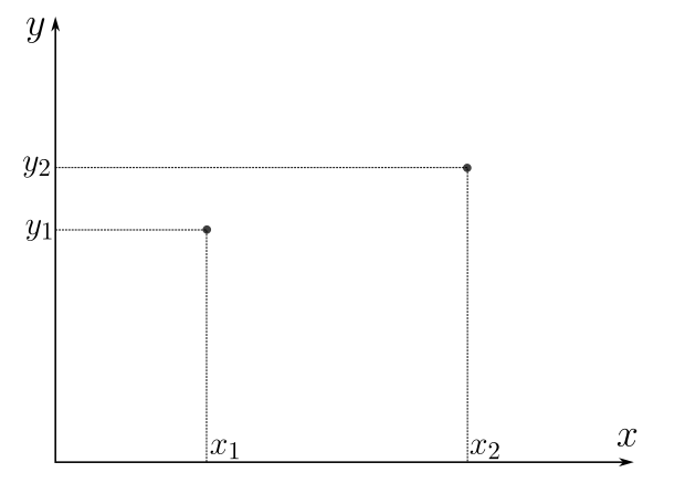
Figure 1: Representation of data. The features are denoted by \(x\), while the response is denoted by \(y\).
In the picture we restrict to two points for the sake of simplicity.
Now, without further information, we could model the data with a straight line, whose functional form is
\begin{equation*} \hat{y}(x) = m x + b. \end{equation*}In the above equation, note firstly the circumflex accent on the \(y\), it means that \(\hat{y}\) is an estimator… that is, does not represent the real data, but it's our way to model the data. The letter \(m\) is the slope of the straight line, and the letter \(b\) indicates the intersection of our estimator function with the vertical axis (\(y\)).
In the figure below we represent with a solid red line a possible estimator function.
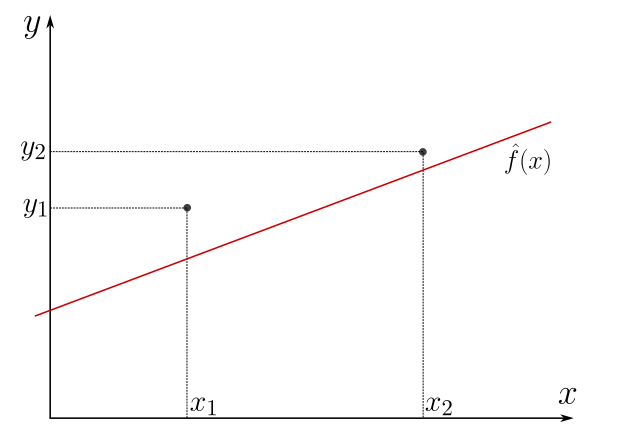
Figure 2: The red line is an example of an estimator function
Hmmm… the red line is not placed where we expected, Is it?
We would like the red line to be as close to the data point as possible, and we were taught that (in Euclidean space) there is always a unique straight line passing through two points. So, the idea is to determine the value of the parameters \(m\) and \(b\) such that the difference between our estimator and the real (expected) values is minimal.
Let us introduce the following notation,
\begin{align*} \hat{y}(x_1) & \equiv \hat{y}_1 = m x_1 + b, \\ \hat{y}(x_2) & \equiv \hat{y}_2 = m x_2 + b. \end{align*}The error of estimation is a notion of how much the estimation differs from the expected output, that in our plot would be the (vertical) distance between the point and the red line. Hence, the total error (or loss function) should be something like the sum of the distances for each value of the predictor variable and the response, mathematically
\begin{align*} \varepsilon = (\hat{y}_1 - y_1) + (\hat{y}_2 - y_2). \end{align*}The error or loss function is a notion that measures the difference of the predicted and expected values. The is no uniqueness in its definition, therefore we can use diverse loss functions depending of the problem of our interest.
The loss function above, \(\varepsilon\), has a problem… the distance can be positive or negative. Hence, there are many ways of adding distances that give vanishing error, illustrated in the figure below. Even worst, this notion of error has no minimum!
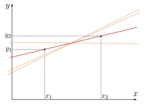
Figure 3: All the red-ish straight lines have vanishing loss (or error) function defined as summed distance. Although we expected the red line, our loss function does not ensure a unique straight line with zero error.
In order to solve these issues, we could try adding the absolute value of the distances,
\begin{align*} \varepsilon = \left| \hat{y}_1 - y_1 \right| + \left| \hat{y}_2 - y_2 \right|, \end{align*}and hence the error is strictly positive and can be minimized. In that case, it is clear that only the red (solid) line that passes through the points has vanishing error.
Consider three data points.
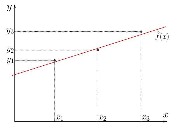
The error defined as the sum of absolute distances cannot vanish… unless the points are colinear (lie on a single straight line). However, we would like to be able of finding systematically the estimator that minimizes the error.
For that end, let us write explicitly the error function,
\begin{align*} \varepsilon & = \sum_i \left| \hat{y}(x_i) - y_i \right| \\ & = \left| m x_1 + b - y_1 \right| + \left| m x_2 + b - y_2 \right| + \left| m x_3 + b - y_3 \right|. \end{align*}Since the loss function depends on the data (\(x_i\) and \(y_i\)), the (unknown) parameters to determine through the optimization are the slope \(m\) and the intersection \(b\). For that we could express the loss function as \(\varepsilon(m,b)\).
Before proceeding to the optimization, note that the minimization (optimization) algorithm requires to derive the function. Deriving the absolute value is hard. In order to avoid the issue of deriving the absolute value, we can propose to change the loss function. Instead of absolute values of the distances, we can square the distances. Our new error function would be
\begin{align*} \varepsilon(m,b) & = \sum_i (\hat{y}_i - y_i) \\ & = \left( m x_1 + b - y_1 \right)^2 + \left( m x_2 + b - y_2 \right)^2 + \left( m x_3 + b - y_3 \right)^2. \end{align*}Let us optimize the function. Reminder: optimizing with respect to a parameter requires that the first derive of the function (with respect to the parameter) vanishes.
The derivatives of the loss function with respect to the parameters are,
\begin{align*} \frac{\partial \varepsilon}{\partial m} & = 2 \sum_i \left( \hat{y}_i - y_i \right) x_i \\ & = 2 \sum_i \left( m x^2_i + b x_i - x_i y_i \right) \\ & = 2 m A + 2 b X - 2 B \end{align*}and
\begin{align*} \frac{\partial \varepsilon}{\partial b} & = 2 \sum_i \left( \hat{y}_i - y_i \right) \\ & = 2 \sum_i \left( m x_i + b - y_i \right) \\ & = 2 m X + 2 N b - 2 Y, \end{align*}where \(N\) is the number of observations in our data, and
\begin{align*} X & = \sum_i x_i, & Y & = \sum_i y_i, \\ A & = \sum_i x^2_i, & B & = \sum_i x_i y_i. \end{align*}Now, the optimization is obtained when
\begin{align*} m A + b X - B & = 0 \\ m X + N b - Y & = 0. \end{align*}Interestingly, we have a determined system of equations (two equations and two unknowns).
From the latter we get that
\begin{align*} b = \frac{1}{N} \left( Y - m X \right). \end{align*}This result can be used in the first equation,
\begin{align*} m = \frac{B - b X}{A} = \frac{N B - X Y + m X^2}{N A}, \end{align*}yielding,
\begin{align*} m = \frac{N B - X Y}{N A - X^2}. \end{align*}Finally, the intersection parameter would be given by
\begin{align*} b = \frac{X^2 Y - B X}{N A - X^2}. \end{align*}Explicitly, using the summation symbols
\begin{align*} m & = \frac{N \sum_i x_i y_i - \sum_i x_i \sum_j y_j}{N \sum_i x^2_i - (\sum_i x_i)^2}, \\ b & = \frac{\sum_i x^2_i \sum_j y_j - \sum_i x_i y_i \sum_j x_j}{N \sum_i x^2_i - (\sum_i x_i)^2}. \end{align*}The above formulas describe the method to adjust a straight line to a set of data, minimizing the error (loss) functions defined by the square distance between the predictions and the observations. This method is known as the Least Square method.