Tossing a coin: a reinforcement learning approach

Tossing a coin is one of the first examples of random events that we experience in our lives (as well as rolling a die, or the rock-paper-scissors game), even as kids we use the method of tossing a coin for decision-making, e.g. selecting an end of a soccer arena.

Nowadays, it has become increasingly difficult to find an actual coin to toss… but we can program our own coin tosser!

In the example below, we assign the values 0 to head and 1 for tail:

from random import randint

value = randint(0,1)
print(f"The lucky winner is: {value}")

The lucky winner is: 0

Easy piecy!

But, what if we agree the winner is the one obtaining two out of three tossing? or three out of five?

import numpy as np

values = np.random.randint(2, size=(5))
print(f"Tossings:\n{values}")

Tossings:
[1 0 0 0 1]

This was useful, but I'm lazy to count the values, specially if we increase the number of tossing. We could use the concept of statistical mode to select the winner, but it is not implemented in numpy. So, we shall use the collections module (other ways can be found in this webpage).

from collections import Counter
import numpy as np

values = np.random.randint(2, size=(51))
print(f"Tossings:\n{values}")
winner = Counter(values).most_common()[0][0]
print(f"The lucky winner is: {winner}")

Tossings:
[0 0 1 0 0 0 1 1 1 1 0 1 0 1 0 0 0 1 0 1 1 0 0 0 0 1 0 0 0 1 0 1 1 1 1 0 1
 1 1 1 1 1 0 0 0 1 1 0 0 1 0]
The lucky winner is: 0

I recommend to read the documentation of Counter, but shortly it is a class that inherits from the dictionary class, and counts the hashtable objects.

So far, we have an algorithm to select an event of the sample space, and finding the item that repeats the most. However, you cannot win a lottery without buying some numbers… Translation: we need an action!

In the code below, I use a random generator available in numpy.random to choose an event from the event space, but also to select an action from the action space. In order to win, the result of tossing the coin has to coincide with your action.

import numpy as np
from numpy.random import default_rng

# instanciate a random generator
rng = default_rng()

state_space = [0, 1]
action_space = [0, 1]

event = rng.choice(state_space)
action = rng.choice(action_space)

if event == action:
    print("You won!")
else:
    print("You losed!")

You losed!

The above can be generalized to many tossing.

import numpy as np
from numpy.random import default_rng

rng = default_rng()
state_space = [0, 1]
action_space = [0, 1]
total, wins = 101, 0

for _ in range(total):
    event = rng.choice(state_space)
    action = rng.choice(action_space)
    if event == action:
        wins += 1

print(f"You won {wins} times out of {total}")

You won 46 times out of 101

We can also repeat out betting algorithm by defining an "epoch" function

import numpy as np
from numpy.random import default_rng

rng = default_rng()
state_space = [0, 1]
action_space = [0, 1]
total = 101


def epoch() -> int:
    wins = 0
    for _ in range(total):
        event = rng.choice(state_space)
        action = rng.choice(action_space)
        if event == action:
            wins += 1
    return wins

winnins = np.array([epoch() for _ in range(200)])
print("Winnings in first 10 epochs:\n", winnins[:10])
print(f"Mean winnins: {winnins.mean()}")

Winnings in first 10 epochs:
 [53 45 58 67 51 49 49 52 49 52]
Mean winnins: 51.11

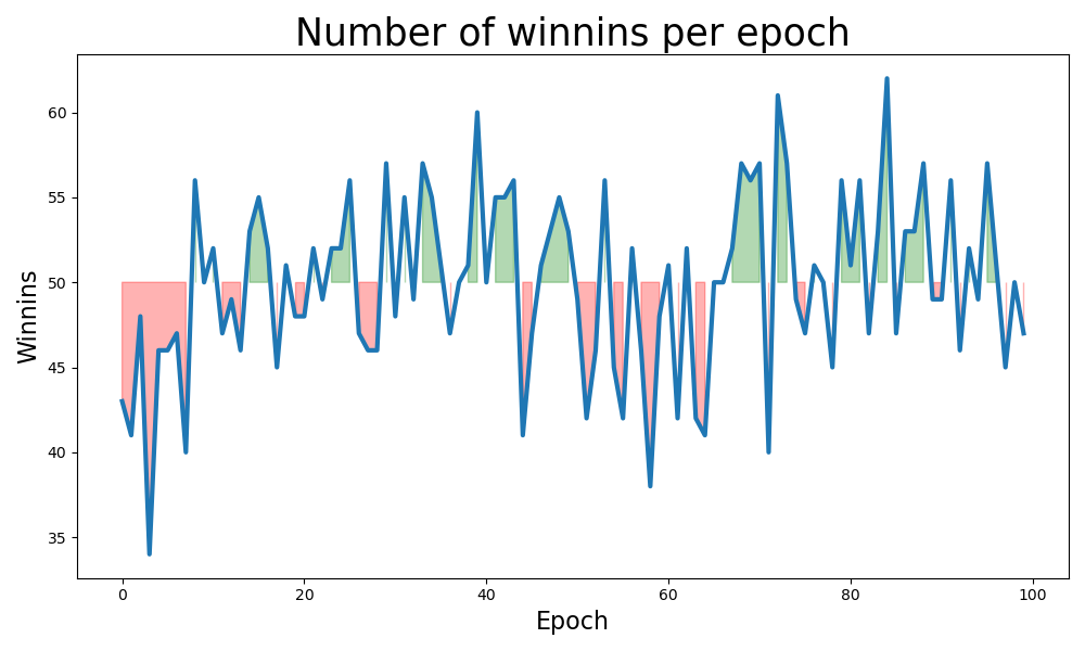
In the code above, we toss the coin 101 times per epoch. We run our algorithm for 200 epochs. From time to time we get lucky and win most of the bets (e.g. 67 out of 101), but the average of winnings is very close to 50%.

Hence, our coin is a fair coin!

Just for fun, I'm plotting the deviation from the expected mean.

import numpy as np
from numpy.random import default_rng
import matplotlib.pyplot as plt

rng = default_rng()
state_space = [0, 1]
action_space = [0, 1]
total, epochs = 101, 100


def epoch() -> int:
    wins = 0
    for _ in range(total):
        event = rng.choice(state_space)
        action = rng.choice(action_space)
        if event == action:
            wins += 1
    return wins

x = np.array(range(epochs))
winnins = np.array([epoch() for _ in range(epochs)])

plt.figure(figsize=(10,6))
plt.plot(x, winnins, lw=3)
plt.fill_between(x, winnins, 50, where=(winnins > 50), color="green", alpha=0.3)
plt.fill_between(x, winnins, 50, where=(winnins < 50), color="red", alpha=0.3)
plt.xlabel("Epoch", fontsize=16)
plt.ylabel("Winnins", fontsize=16)
plt.title("Number of winnins per epoch", fontsize=25)
plt.tight_layout()
plt.savefig(filename)
return filename

What would change if our coin is biased?

The effect of a biased coin can be expressed by a modification to the space of states, for example [0, 0, 0, 1] instead of [0, 1]. So, let find out!

import numpy as np
from numpy.random import default_rng

rng = default_rng()
state_space = [0, 0, 0, 1]
action_space = [0, 1]
total = 101


def epoch() -> int:
    wins = 0
    for _ in range(total):
        event = rng.choice(state_space)
        action = rng.choice(action_space)
        if event == action:
            wins += 1
    return wins

winnins = np.array([epoch() for _ in range(200)])
print("Winnings in first 10 epochs:\n", winnins[:10])
print(f"Mean winnins: {winnins.mean()}")

Winnings in first 10 epochs:
 [52 46 43 54 44 51 54 53 46 49]
Mean winnins: 50.425

WHAT???????… It was not what I expected!

Let's calculate the expected value,

\begin{equation} \label{eq:1} E[\mathrm{win}] = \frac{3}{4} \times \frac{1}{2} + \frac{1}{4} \times \frac{1}{2} = \frac{4}{8} = \frac{1}{2}. \end{equation}

Wow, interestingly, the randomly selected action wash out the bias of the state space.

Learning from observation

In the later experience, the probability of winning was a half. Essentially driven by the fact that our action space was not modified. However, if we have the hunch that the space of events is not fair, we might bias our action choice.

import numpy as np
from numpy.random import default_rng

rng = default_rng()
state_space = [0, 0, 0, 1]
total = 101


def epoch() -> int:
    wins = 0
    action_space = [0, 1]
    for _ in range(total):
        event = rng.choice(state_space)
        action = rng.choice(action_space)
        action_space.append(event)
        if event == action:
            wins += 1
    return wins

winnins = np.array([epoch() for _ in range(200)])
print("Winnings in first 10 epochs:\n", winnins[:10])
print(f"Mean winnins: {winnins.mean()}")

Winnings in first 10 epochs:
 [70 51 60 57 55 63 65 71 66 68]
Mean winnins: 62.295

Now we are talking!

What happened? As we update our action space, the proportion of head and tails in the action space resemble the ones in the state space. Hence, the expected value is

\begin{equation} \label{eq:2} E[\mathrm{win}] = \frac{3}{4} \times \frac{3}{4} + \frac{1}{4} \times \frac{1}{4} = \frac{5}{8} = 0.625. \end{equation}

The expected and the simulated results are very similar.

Note that even if we where able of rising our winning rate, it is still below the actual bias rate (75% in our case of study).

In order to increase our winning rate as much as to the bias rate, we would have to bet to the most common value in our state space. Since we have no access to the state space a priori, we have to induce it from experience through counting. We already used the .most_common() function from the collections.Count module, so let's implement this last scenario:

import numpy as np
from numpy.random import default_rng
from collections import Counter

rng = default_rng()
state_space = [0, 0, 0, 1]
total = 101


def epoch() -> int:
    wins = 0
    action_space = [0, 1]
    for _ in range(total):
        event = rng.choice(state_space)
        action = Counter(action_space).most_common()[0][0]
        action_space.append(event)
        if event == action:
            wins += 1
    return wins

winnins = np.array([epoch() for _ in range(200)])
print("Winnings in first 10 epochs:\n", winnins[:10])
print(f"Mean winnins: {winnins.mean()}")

Winnings in first 10 epochs:
 [76 72 79 74 71 75 74 72 80 75]
Mean winnins: 75.005