Exploring numerical integration with numpy

A typical exercise in calculus is the calculation of the integral of a function.

The geometrical interpretation of the integral is the "area below the curve". I wanted to use numpy to calculate the approximate value of the integral of a function.

Consider the sine function, sin(x), and let's calculate its integral in the interval \((0, \pi)\).

from sympy import Symbol, sin, integrate, pi

x = Symbol('x')
value = integrate(sin(x), (x, 0, pi))
print(f"Result: {value}")

Result: 2

We can use numpy to calculate an approximate value.

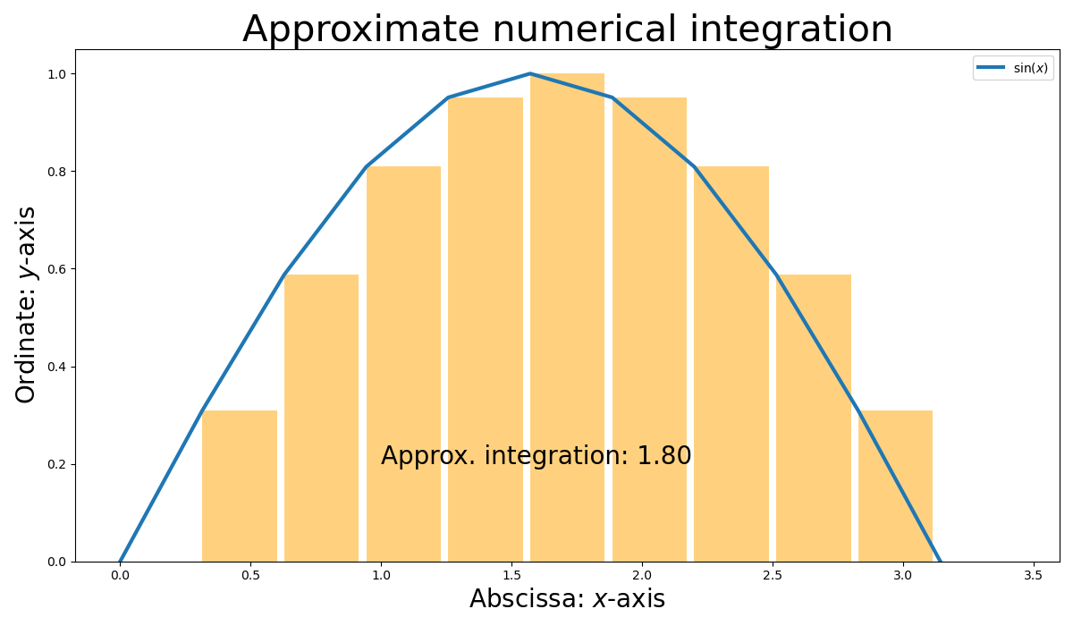
import numpy as np

a, b, steps = 0, np.pi, 11
dx = (b - a) / steps

x = np.linspace(a, b, steps)
result = np.sin(x).sum() * dx
print(f"Num. integration = {result:.2f}")

Num. integration = 1.80

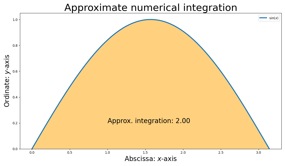
Let's try to visualize the integration process.

import numpy as np
import matplotlib.pyplot as plt

a, b, steps = 0, np.pi, 11
dx = (b - a) / steps
x = np.linspace(a, b, steps)
y = np.sin(x)
result = y.sum() * dx

plt.figure(figsize=(12,7))
plt.plot(x, y, lw=3, label=r"$\sin(x)$")
plt.bar(x, y, width=dx, align='edge', color="orange", alpha=.5)
plt.title("Approximate numerical integration", fontsize=30)
plt.xlabel(r"Abscissa: $x$-axis", fontsize=20)
plt.ylabel(r"Ordinate: $y$-axis", fontsize=20)
plt.text(1, 0.2, f"Approx. integration: {result:.2f}", fontsize=20)
plt.legend()
plt.tight_layout()
plt.savefig(filename)
return filename

Note that if we increase the number of steps, the numerical result tends to the analytical one:

import numpy as np
import matplotlib.pyplot as plt

a, b, steps = 0, np.pi, 101
dx = (b - a) / steps
x = np.linspace(a, b, steps)
y = np.sin(x)
result = y.sum() * dx

plt.figure(figsize=(12,7))
plt.plot(x, y, lw=3, label=r"$\sin(x)$")
plt.bar(x, y, width=dx, align='edge', color="orange", alpha=.5)
plt.title("Approximate numerical integration", fontsize=30)
plt.xlabel(r"Abscissa: $x$-axis", fontsize=20)
plt.ylabel(r"Ordinate: $y$-axis", fontsize=20)
plt.text(1, 0.2, f"Approx. integration: {result:.2f}", fontsize=20)
plt.legend()
plt.tight_layout()
plt.savefig(filename)
return filename

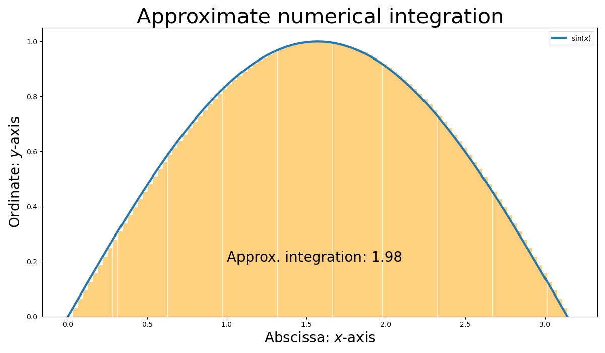
.. or even tinier:

import numpy as np
import matplotlib.pyplot as plt

a, b, steps = 0, np.pi, 1001
dx = (b - a) / steps
x = np.linspace(a, b, steps)
y = np.sin(x)
result = y.sum() * dx

plt.figure(figsize=(12,7))
plt.plot(x, y, lw=3, label=r"$\sin(x)$")
plt.bar(x, y, width=dx, align='edge', color="orange", alpha=.5)
plt.title("Approximate numerical integration", fontsize=30)
plt.xlabel(r"Abscissa: $x$-axis", fontsize=20)
plt.ylabel(r"Ordinate: $y$-axis", fontsize=20)
plt.text(1, 0.2, f"Approx. integration: {result:.2f}", fontsize=20)
plt.legend()
plt.tight_layout()
plt.savefig(filename)
return filename