A first attempt to predict tendencies in stockmarket

In python, the library yfinance allows us to download financial data from Yahoo finance.

Since I'm currently doing a certification in Generic AI for finance, I created a folder to store and manage programs related to my incursion in the field, and use uv to install the necessary packages (in the group dev)

mkdir genai-finance
cd !$
uv init --bare
uv add --dev yfinance curl_cffi scikit-learn

The program (which I called basic.py) starts loading the libraries, in this example I'll use a RandomForestClassifier algorithm as ML model.

import yfinance as yf
import pandas as pd
from sklearn.ensemble import RandomForestClassifier
from sklearn.model_selection import train_test_split

The yfinance module is used to download the data,

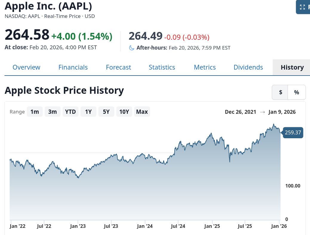
data = yf.download("AAPL", start="2022-01-01", end="2026-01-01")

The downloaded data is stored as a pandas dataframe (you can use the command print(f"Data datatype: {type(data)}") to check it).

I started exploring the data, using

data.info,
data.describe(),
data.columns,
data.notna().sum(), etc.

I note that the columns used the pd.MultiIndex property, and it was preferable (for me) to change it, using the momentum I rename the columns to a lowercase version of their names.

if isinstance(data.columns, pd.MultiIndex):
    data.columns = data.columns.get_level_values(0)

data = data.rename(columns={
    "Open": "open",
    "High": "high",
    "Low": "low",
    "Close": "close",
    "Volume": "volume"
})

Then, I converted the indices to datetime datatype and ensure the dataframe is sorted correctly:

data.index = pd.to_datetime(data.index)
df = data.sort_index()

Now, we define some features:

return: the decimal expression of the percentage return, with respect to the previous day,
ma10: the average of the stock price over a 10 days window, and
target: a binary index with values 1 if the return is positive and 0 if the return is negative.

These are implemented using the .pct_change() and .rolling(window=10) methods of the pandas dataframe:

df['return'] = df['close'].pct_change()
df['ma10'] = df['close'].rolling(window=10).mean()
df["target"] = (df["return"] > 0).astype(int)
df.dropna(inplace=True)

The machine learning process starts now. We split our data into train and test, define the model, train it with the train data, and use it to predict on the test data:

features = ["open", "high", "low", "close", "volume", "ma10"]
X = df[features]
y = df["target"]

X_train, X_test, y_train, y_test = train_test_split(
    X, y, test_size=0.1, shuffle=False
)

model = RandomForestClassifier(
    n_estimators=100,
)
model.fit(X_train, y_train)

accuracy = model.score(X_test, y_test)
print(f"Test Accuracy: {accuracy:.2f}")

I was very excited about the analysis! However, the accuracy round the 50%. This is as bad as tossing a coin to decide whether we want to sell of buy stocks on a given day 😕. Not promising!

Let's wait to see how other techniques improve the performance.