First investing simulating with backtrader

What is backtrader?

A feature-rich Python framework for backtesting and trading

backtrader allows you to focus on writing reusable trading strategies, indicators and analyzers instead of having to spend time building infrastructure.

Imagine that you hire a trader. In your first communication you describe to her/him, how much money you want to invest, your financial goals, where you want to invest, but also you design an investing strategy (which depends on your goal and investor profile).

Backtrader allows you to simulate the performance of your strategy!

Since I've been playing with yfinance to download and analyze stockmarket data, my workflow continues from there.

Let's start loading the libraries

import yfinance as yf
import pandas as pd
import backtrader as bt
from datetime import datetime

and defining (or reusing) the functions to retrieve, clean and enhance the data with financial features

def retrieve_clean_data(symbol: str, start_date: str, end_date: str):
    """
    Retrieve the stockmarket data:
    - symbol: Stock abbreviation, e.g. "AAPL", "MSFT"
    - start_date: in format YYYY-MM-DD
    - end_date: in format YYYY-MM-DD

    Returns a pandas DataFrame
    """
    data = yf.download(symbol, start=start_date, end=end_date)

    if isinstance(data.columns, pd.MultiIndex):
        data.columns = data.columns.get_level_values(0)

    data = data.rename(columns={
        "Open": "open",
        "High": "high",
        "Low": "low",
        "Close": "close",
        "Volume": "volume"
    })

    data.index = pd.to_datetime(data.index)
    return data.sort_index()


def feature_engineering(df: pd.DataFrame) -> pd.DataFrame:
    """
    Feature Engineering. Creates the features:
    - return: decimal equivalent of percentage change
    - ma10: moving average over 10 days
    - target: variable indicating raising (1) or falling (0)
      of the share price.
    """
    df['return'] = df['close'].pct_change()
    df['ma10'] = df['close'].rolling(window=10).mean()
    df["target"] = (df["return"] > 0).astype(int)
    df.dropna(inplace=True)
    return df

With the above, I shall be able of getting our data.

The next step is to define our investment strategy, which would be a backtrader.Strategy class.

class FirstStrategy(bt.Strategy):

    def log(self, txt, dt=None):
        ''' Logging function fot this strategy'''
        dt = dt or self.datas[0].datetime.date(0)
        print('%s, %s' % (dt.isoformat(), txt))

    def __init__(self):
        self.dataclose = self.datas[0].close

    def next(self):
        self.log('Close, %.2f' % self.dataclose[0])

        if self.dataclose[0] < self.dataclose[-1]:
            # current close less than previous close
            if self.dataclose[-1] < self.dataclose[-2]:
                # previous close less than the previous close
                # BUY, BUY, BUY!!! (with all possible default parameters)
                self.log('BUY CREATE, %.2f' % self.dataclose[0])
                self.buy()

How does it work? Our trader will go through the data (note that at a given point in the data, the trader denotes with index zero, [0], the current moment in the analysis) using the next method. In the next method, we decide to buy shares if the stock price (at close) has decline the last two days.

The __init__ method defines the dataclose instance using the closing prices from the data. The log method prints the current date of the simulation, together with a given text.

Finally, the main part of the simulation.

def main():
    symbol = "META"
    start_date = datetime(year=2021,
                          month=1,
                          day=1)
    end_date = datetime(year=2026,
                        month=2,
                        day=1)
    df = retrieve_clean_data(symbol, start_date, end_date)
    df = feature_engineering(df)
    # Convert DataFrame to backtrader data feed
    # Ensure the DataFrame has the required columns
    data = bt.feeds.PandasData(
        dataname=df,
        datetime=None,  # Adjust this to match your date column name
        open='open',
        high='high',
        low='low',
        close='close',
        volume='volume',
        openinterest=-1  # -1 indicates no open interest
    )

    # Now our bt Cerebro
    cerebro = bt.Cerebro()
    cerebro.addstrategy(FirstStrategy)
    cerebro.broker.set_cash(5_000)
    print(f"Initial portfolio value: {cerebro.broker.getvalue():.2f}")
    cerebro.adddata(data)
    cerebro.run()
    print(f"Final portfolio investment: {cerebro.broker.getvalue():.2f}")


if __name__ == "__main__":
    main()

The relevant thing is that we instantiate a Cerebro() (which plays the role of our broker!), add the strategy and set the amount of our investment.

Then, we run our simulation and retrieve the final value of our investment.

The result:

.
.
.
2026-01-02, BUY CREATE, 650.41
2026-01-05, Close, 658.79
2026-01-06, Close, 660.62
2026-01-07, Close, 648.69
2026-01-08, Close, 646.06
2026-01-08, BUY CREATE, 646.06
2026-01-09, Close, 653.06
2026-01-12, Close, 641.97
2026-01-13, Close, 631.09
2026-01-13, BUY CREATE, 631.09
2026-01-14, Close, 615.52
2026-01-14, BUY CREATE, 615.52
2026-01-15, Close, 620.80
2026-01-16, Close, 620.25
2026-01-20, Close, 604.12
2026-01-20, BUY CREATE, 604.12
2026-01-21, Close, 612.96
2026-01-22, Close, 647.63
2026-01-23, Close, 658.76
2026-01-26, Close, 672.36
2026-01-27, Close, 672.97
2026-01-28, Close, 668.73
2026-01-29, Close, 738.31
2026-01-30, Close, 716.50
Final portfolio investment: 12948.17

It worked! And the investment has increased 150% 🤑

BUT WAIT!!!

Do you remember the visualization of share prices?

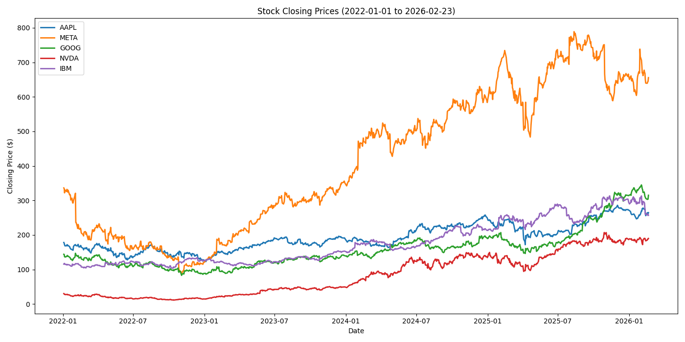
Note that the performance of the META shares is about 130%. I'll be returning to this point after further reading and analysis.