ndarray: a special data type for numerical data

The library numpy offers various ways to create arrays.

A simple method is to transform a list into an ndarray, but there are other forms to get them:

import numpy as np
a = np.array([0, 1, 2, 3.5, 4.2, 10])
print("a =", a)
b = np.linspace(0, 1, 11)
print("b =", b)
c = np.arange(0, 1.05, 0.1)
print("c =", c)
d = np.zeros(5)
print("d =", d)
e = np.ones(6)
print("e =", e)
f = np.random.rand(5)
print("f =", f)
g = np.random.randint(11, size=6)
print("g =", g)

a = [ 0.   1.   2.   3.5  4.2 10. ]
b = [0.  0.1 0.2 0.3 0.4 0.5 0.6 0.7 0.8 0.9 1. ]
c = [0.  0.1 0.2 0.3 0.4 0.5 0.6 0.7 0.8 0.9 1. ]
d = [0. 0. 0. 0. 0.]
e = [1. 1. 1. 1. 1. 1.]
f = [0.5451996  0.49368761 0.48197987 0.28080124 0.18046084]
g = [ 3  5  1 10  8  1]

All of the above example are similar to a list, and are enter into the class of one-dimensional array. However, ndarray allows us to create higher-dimensional arrays.

Here are a couple of examples of ways to create two-dimensional ndarray:

import numpy as np
a = np.array([[1.3, 4], [9.3, -3.14]])
print("a =\n", a)
b = np.random.rand(4,5)
print("b =\n", b)
c = np.random.randint(11, size=(4,5))
print("c =\n", c)
d = np.eye(4)
print("d =\n", d)
e = np.zeros((3,4))
print("e =\n", e)
f = np.ones((2,5))
print("f =\n", f)

a =
 [[ 1.3   4.  ]
 [ 9.3  -3.14]]
b =
 [[0.5391786  0.05398241 0.21687336 0.28755768 0.62844929]
 [0.78871333 0.06122128 0.46469304 0.20521034 0.74049581]
 [0.33120551 0.8659041  0.23759993 0.9672616  0.65304733]
 [0.5042783  0.20098257 0.7937683  0.03892913 0.32799822]]
c =
 [[ 1  0  6  4  8]
 [ 0  1  9  6  1]
 [10  3  9  2  1]
 [ 5  0  6  7  9]]
d =
 [[1. 0. 0. 0.]
 [0. 1. 0. 0.]
 [0. 0. 1. 0.]
 [0. 0. 0. 1.]]
e =
 [[0. 0. 0. 0.]
 [0. 0. 0. 0.]
 [0. 0. 0. 0.]]
f =
 [[1. 1. 1. 1. 1.]
 [1. 1. 1. 1. 1.]]

Knowing how to build ndarray, we have to start working with them.

In python each data type admits transformation under a set of arithmetic operations, as addition (+) or multiplication (*). Let's illustrate the difference between list and ndarray:

import numpy as np
a_list = [1, 2, 3]
b_list = [4, 5, 6]
print("Addition of list:", a_list + b_list)
print("Addition of ndarray:", np.array(a_list) + np.array(b_list))

Addition of list: [1, 2, 3, 4, 5, 6]
Addition of ndarray: [5 7 9]

The above code block can be resumed into two pictures:

• The addition operation concatenates list

  

• The addition operation of ndarray sums element-wise:

  

If you are custom to vector algebra, the addition of ndarray resembles the addition of vectors. In fact, numpy has been developed to behave in that way.

Let's try other operations:

import numpy as np
a_list = [1, 2, 3]
b_list = [4, 5, 6]
print("Addion of ndarray:", np.array(a_list) + np.array(b_list))
print("Subtraction of ndarray:", np.array(a_list) - np.array(b_list))
print("Multiplication of ndarray:", np.array(a_list) * np.array(b_list))
print("Division of ndarray:", np.array(a_list) / np.array(b_list))
print("Power of ndarray:", np.array(a_list) ** np.array(b_list))

Addion of ndarray: [5 7 9]
Subtraction of ndarray: [-3 -3 -3]
Multiplication of ndarray: [ 4 10 18]
Division of ndarray: [0.25 0.4  0.5 ]
Power of ndarray: [  1  32 729]

When we study vectors on three-dimensional space, there are two products between vectors (which do not coincide with the product in the previous section):

• Scalar product of vectors, also known as dot product, is calculated in numpy with the function np.dot(a, b)

• Vector product of vectors, known as cross product, calculated in numpy with the function np.cross(a,b).

  It is worth mentioning that the dot product can be defined in vector spaces of any dimension, while the cross product is proper of three-dimensional vector spaces.

  In addition, one has to be aware that the functions np.dot() and np.cross() might be applied to higher-dimensional arrays.

The operations presented in the section Arithmetic of ndarray, act element-wise. This is the expected action when we want to perform numerical calculations. numpy redefines many (if not all) of the mathematical functions in the math module, to act over ndarray element-by-element. Such functions are named U-functions.

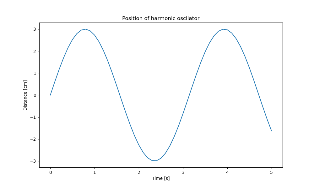
To show how to use them, consider the physical system of mass-spring. The distance of the mass, respect to the equilibrium, is modeled by the equation

where \(A\) is the maximum deformation of the spring (or amplitude), \(\omega\) is the angular frequency and \(\varphi\) is the phase (related to the initial conditions of the system).

For \(A=3\), \(\omega = 2\) and \(\varphi = 0\), the calculation is given by

import numpy as np
times = np.linspace(0, 5, 51)
distances = 3 * np.sin(2 * times)
print("Distances = ", distances)

Distances =  [ 0.          0.59600799  1.16825503  1.69392742  2.15206827  2.52441295
  2.79611726  2.95634919  2.99872081  2.92154289  2.72789228  2.42548921
  2.02638954  1.54650412  1.00496445  0.42336002 -0.17512243 -0.76662331
 -1.32756133 -1.83557367 -2.27040749 -2.61472732 -2.85480622 -2.98107301
 -2.98849383 -2.87677282 -2.65036397 -2.31829346 -1.89379991 -1.39380654
 -0.83824649 -0.24926821  0.34964761  0.93462409  1.48234005  1.9709598
  2.38100359  2.69612429  2.90375902  2.99563004  2.96807474  2.82219167
  2.56379672  2.20319129  1.75475158  1.23635546  0.66866974  0.07432628
 -0.52298034 -1.09943739 -1.63206333]

However, it is simpler to plot the results:

import numpy as np
import matplotlib.pyplot as plt
times = np.linspace(0, 5, 51)
distances = 3 * np.sin(2 * times)

plt.figure(figsize=(10,6))
plt.plot(times, distances)
plt.xlabel("Time [s]")
plt.ylabel("Distance [cm]")
plt.title("Position of harmonic oscilator")
plt.savefig(filename)
return filename

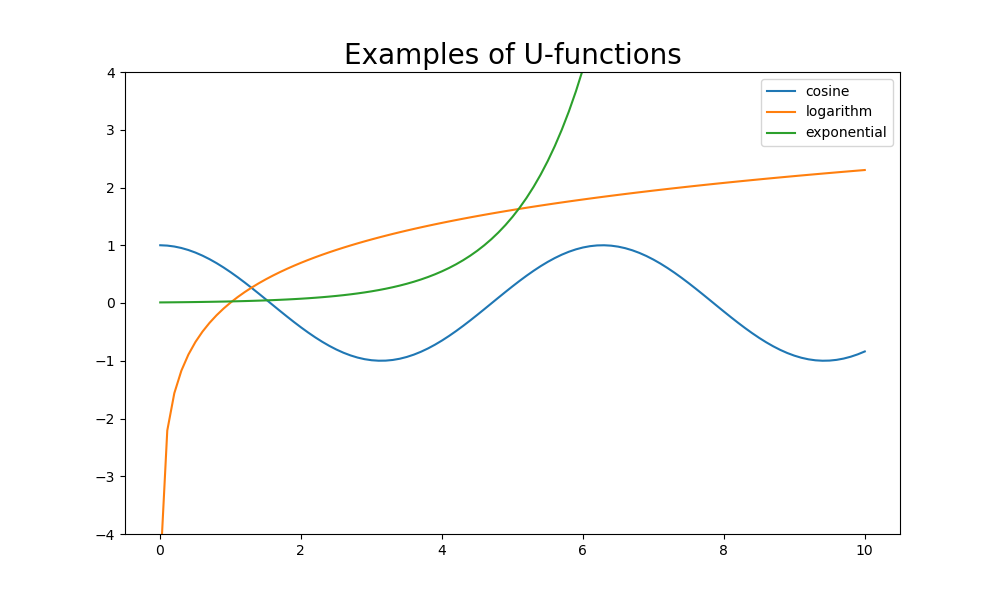
There are many other u-functions:

import numpy as np
import matplotlib.pyplot as plt
t = np.linspace(0.01, 10, 101)

plt.figure(figsize=(10,6))
plt.plot(t, np.cos(t), label="cosine")
plt.plot(t, np.log(t), label="logarithm")
plt.plot(t, 1/100 * np.exp(t), label="exponential")
plt.title("Examples of U-functions", fontsize=20)
plt.legend()
plt.ylim([-4,4])
plt.savefig(filename)
return filename